


In today’s world of data analysis, variance analysis has become an important tool to visualize changes in data over time. By comparing actual data with projected or budgeted data, businesses can identify and understand the reasons behind fluctuations in their financial or operational performance. One effective way of visualizing variances in data is to create an integrated variance column chart in Microsoft Excel.
Table of Contents
Understanding the importance of variance analysis in data visualization
Variance analysis is a valuable technique for any business to uncover what is driving changes in their data over time. This type of analysis helps businesses to understand whether or not they are meeting their goals and to identify which factors are contributing to or detracting from their performance. For example, if a business or department’s sales have significantly increased or decreased over a particular period of time, variance analysis can help identify the underlying factors that are influencing these changes. This information can be used to make informed decisions about how to improve the business’ performance moving forward.
Moreover, variance analysis can also help businesses to identify trends and patterns in their data that may not be immediately apparent. By analyzing the variances between different data points, businesses can gain insights into the relationships between different factors and how they are affecting overall performance. This can be particularly useful in identifying areas where the business may be underperforming or where there may be opportunities for growth and improvement.
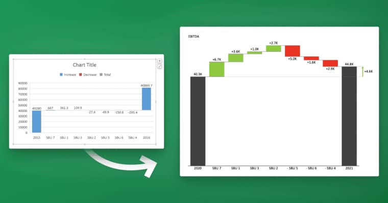
Step-by-step guide to creating a variance column chart in Excel
To create an integrated variance column chart in Excel, follow these simple steps:
- Select the data set you want to represent in your chart, including actual and budgeted values for each period.
- Click on the “Insert” tab, then select “Column” from the “Charts” group.
- In the dropdown options, select the “Clustered Column” chart type.
- Right-click the actual series in your chart and select “Change Series Chart Type”.
- Select “Combo” from the options and choose the secondary axis.
- Select the budget series and format it. Change the fill color to white so that it shows the variance column.
- Finish formatting by selecting the chart and using the design tab. Change colors, add titles, and select other customizations as desired.
Creating a variance column chart in Excel can be a useful tool for analyzing the differences between actual and budgeted values. This type of chart can help you identify areas where you may need to adjust your budget or spending habits.
It’s important to note that when creating a variance column chart, you should ensure that your data is accurate and up-to-date. This will help you make informed decisions based on the information presented in the chart.
Choosing the right data set for your integrated variance chart
The data set you choose for your integrated variance chart must have actual and budgeted values for the same periods of time. This may require some cleaning up of data and careful attention to the formatting of dates and other relevant data points. It’s important to ensure that you are comparing like-with-like so that the chart is accurate, and any significant deviations in the data are easily identifiable.
Additionally, it’s important to consider the source of the data and whether it is reliable. If the data is coming from multiple sources, it’s important to ensure that the data is consistent and that any discrepancies are resolved before creating the chart. It’s also important to consider the frequency of the data – if the data is only available on a monthly basis, for example, it may not be suitable for creating a chart that requires more granular data. By carefully selecting and preparing your data set, you can ensure that your integrated variance chart provides accurate and meaningful insights into your business performance.
Tips for formatting and customizing your variance chart
One tip for formatting your variance chart is to use contrasting colors for your actual and budgeted data, and to utilize white or neutral colors for your variance columns. This will help your audience to quickly and easily identify where the variances lie. Additionally, consider adding titles and labels to your chart to make it easier to understand. Take some time to explore other chart customization options to make your chart look professional and visually appealing.
Another important tip for formatting your variance chart is to ensure that the chart is easy to read and understand. This can be achieved by using clear and concise language in your titles and labels, and by avoiding cluttering the chart with too much information. It is also important to choose the right type of chart for your data, as different types of charts are better suited for different types of data.
Finally, consider adding annotations or callouts to your chart to highlight important data points or trends. This can help to draw your audience’s attention to key insights and make your chart more engaging. However, be careful not to overdo it with annotations, as too many can make the chart look cluttered and confusing.
Analyzing and interpreting your integrated variance chart
Once you have created your integrated variance chart, it is important to take the time to analyze and interpret the data. Look for any significant changes or trends and consider what factors may have contributed to these deviations. Remember to consider external factors as well, such as general economic conditions, changes in the industry or market, or regulatory changes. Understanding these factors can help you to make strategic decisions that will benefit your business.
Another important aspect to consider when analyzing your integrated variance chart is the impact of internal factors. Look at your company’s operations and processes to identify any areas where improvements can be made. This could include streamlining processes, reducing waste, or improving communication between departments. By addressing these internal factors, you can reduce variance and improve overall performance.
It is also important to regularly review and update your integrated variance chart. As your business evolves and changes, so too will the factors that contribute to variance. By regularly reviewing and updating your chart, you can ensure that you are making informed decisions based on the most up-to-date information available.
Using pivot tables to create an integrated variance chart in Excel
You can also use pivot tables to create an integrated variance chart in Excel. This method is especially useful if you have large sets of data that require extensive calculation and filtering. Pivot tables allow you to easily organize and summarize your data, making your integrated variance chart more effective and efficient.
One of the benefits of using pivot tables to create an integrated variance chart is that you can easily update the chart as new data is added. This means that you don’t have to manually adjust the chart every time new data is entered, saving you time and effort. Additionally, pivot tables allow you to quickly identify trends and patterns in your data, which can help you make more informed business decisions.
However, it’s important to note that creating an integrated variance chart using pivot tables can be complex, especially if you’re not familiar with Excel’s advanced features. It’s recommended that you take some time to learn about pivot tables and practice using them before attempting to create an integrated variance chart. There are many online resources and tutorials available that can help you get started.
Comparing actual vs budgeted data in an integrated variance chart
In an integrated variance column chart, the actual data is visually represented by a solid color column, while the budgeted data is represented by a dashed line column. The variance between the two can be shown in a separate column or chart. Comparing actual vs budgeted data allows you to determine if you are meeting your financial goals, and to identify any discrepancies or issues that may require attention.
It is important to note that when comparing actual vs budgeted data, it is essential to use accurate and up-to-date information. This means regularly updating your budget and tracking your actual expenses to ensure that the data being compared is reliable. Additionally, it is helpful to analyze the variances between actual and budgeted data over time to identify trends and make informed decisions about future financial planning.
How to use conditional formatting to highlight variances in your chart
Conditional formatting is a powerful tool that can help you to highlight specific data points in your integrated variance chart. For example, you can use conditional formatting to highlight any variances that exceed a certain threshold or are outside of a specific range. This can help you to quickly identify areas that require further investigation or action.
Another way to use conditional formatting in your chart is to highlight trends over time. You can set up conditional formatting rules to show if a data point is increasing, decreasing, or staying the same over a period of time. This can help you to identify patterns and make informed decisions based on the data.
It’s important to note that conditional formatting can be applied to various types of charts, including bar charts, line charts, and pie charts. By using conditional formatting, you can make your data more visually appealing and easier to understand, which can ultimately lead to better decision-making.
Best practices for sharing and presenting your integrated variance chart
When sharing your integrated variance chart with others, it’s important to keep in mind who your audience is and what their level of understanding of the data may be. Be prepared to explain any technical terms or concepts, and consider using annotations or callouts to highlight important trends or data points. Additionally, consider including other supporting materials such as a summary of key findings or a written report to provide additional context and analysis.
In conclusion, creating an integrated variance column chart in Excel is a useful way to visualize data changes over time. Through variance analysis, businesses can gain a better understanding of their performance and identify opportunities for improvement. By following best practices for formatting and customizing your chart, you can create an effective tool that helps you and your team make informed decisions based on the data.
Another important consideration when sharing your integrated variance chart is to ensure that the chart is visually appealing and easy to read. Use contrasting colors and clear labels to make it easy for your audience to understand the data. Avoid cluttering the chart with too much information, as this can make it difficult to interpret.
Finally, it’s important to keep your integrated variance chart up-to-date. As new data becomes available, update your chart to reflect the latest information. This will ensure that your team is always working with the most current data and can make informed decisions based on the latest insights.