How to Pull Information From Another Sheet in Excel
Excel is a powerful tool for handling large sets of data. It allows users to organize information in a structured way and provides tools for analyzing and manipulating data. One of the most valuable features of Excel is its ability to reference data from other sheets within a workbook or even from another workbook. This allows users to easily pull information from different sources and consolidate it into one location for more straightforward analysis. In this article, we'll explore the different ways to pull information from another sheet in Excel and provide tips for troubleshooting common issues.
Understanding the Basics of Referencing in Excel
Before we dive into the different methods of pulling information from another sheet, it's essential to understand the basics of referencing in Excel.
A reference is simply a way of identifying a cell or range of cells in a worksheet. References can be absolute, meaning they always point to a specific cell or relative based on a specific position relative to the cell containing the reference.
The syntax is straightforward when referencing cells or ranges in the same worksheet. For example, to reference the cell A1, you can type "=A1" into another cell. However, when referencing cells or ranges in a different worksheet, you need to include the sheet name in the reference.
It's also important to note that when referencing cells or ranges in a different workbook, you must include both the sheet and the workbook names in the reference. This is known as an external reference. External references can be helpful when you need to pull data from multiple workbooks into a single worksheet or when you want to link data between workbooks.
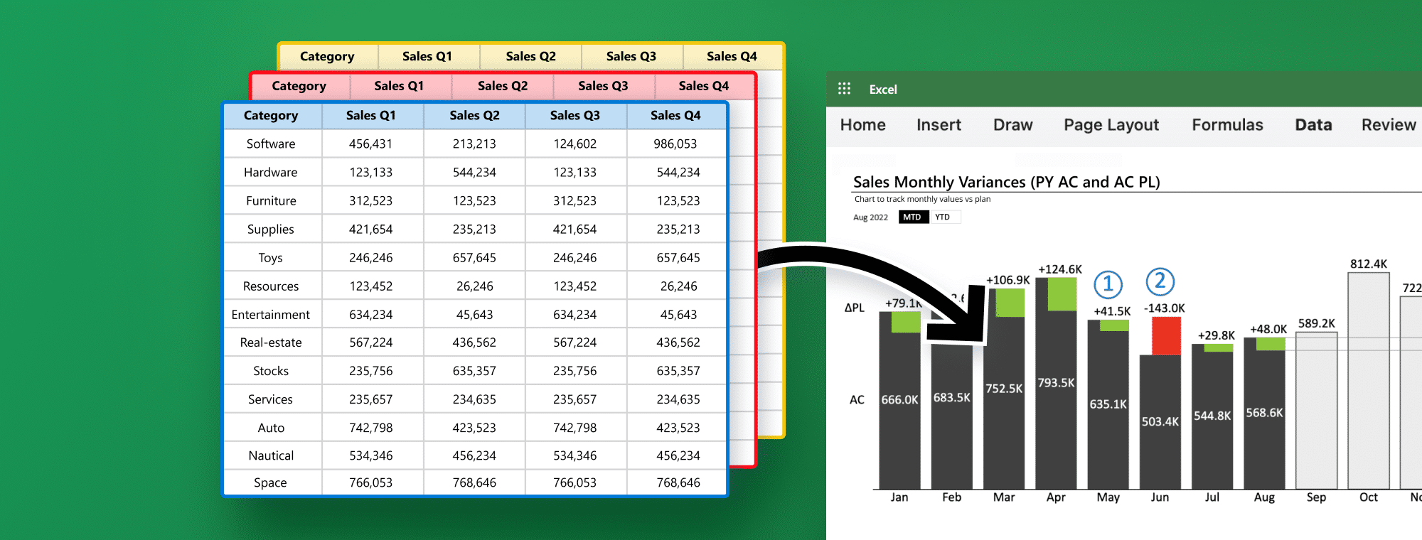
Imagine consolidating data to build an interactive dashboard (with cross-visual filtering) inside your Excel workbook with Zebra BI Charts and Tables.
Using the INDEX Function to Retrieve Information from Another Sheet
The INDEX function is one of the most versatile functions in Excel and can be used to return a specific value from a table or range of cells. It's handy for retrieving data from another sheet in a workbook. The syntax for the INDEX function is =INDEX(array,row_num,column_num). The array argument is the range of cells from which you want to retrieve the data. The row_num and column_num arguments indicate the position of the data you want to retrieve within the array.
You'll need to include the sheet name in the array argument to use the INDEX function to retrieve data from another sheet. For example, if you want to retrieve data from Sheet2 in a workbook, the syntax would be =INDEX(Sheet2!A1:B10,2,1). This will return the value in the second row and first column of the range A1:B10 in Sheet 2.
It's important to note that the INDEX function can also be combined with other functions, such as MATCH and IF, to create more complex formulas. For example, you can use the MATCH function to find the position of a specific value in a range and then use the INDEX function to retrieve the corresponding value from another sheet. This can be particularly useful when working with large datasets or when you need to perform calculations based on data from multiple sheets.
Using the VLOOKUP Function to Retrieve Data from Another Sheet
The VLOOKUP function is another powerful tool for retrieving data from another sheet in a workbook. It allows you to search for a specific value in a table and return a corresponding value from a specified column. The syntax for the VLOOKUP function is =VLOOKUP(lookup_value,table_array,col_index_num,range_lookup). The lookup_value is the value you want to search for, the table_array is the range of cells that contains the table, the col_index_num is the column number that contains the value you want to retrieve, and the range_lookup argument indicates whether you want to find an exact match or an approximate match.
To use the VLOOKUP function to retrieve data from another sheet, you'll need to include the sheet name in the table_array argument. For example, if you want to retrieve data from Sheet2 in a workbook, the syntax would be =VLOOKUP(A1,Sheet2!A1:B10,2,FALSE). This will search for the value in cell A1 in the range A1:B10 in Sheet 2 and return the corresponding value from the second column.
Check out Excel templates you can use once you have pulled the data together in our Excel Templates Library.
How to Use the MATCH Function to Find Data in Another Sheet
The MATCH function is another powerful tool for working with data in Excel. It allows you to search for a specific value in a range of cells and return its position within the range. The syntax for the MATCH function is =MATCH(lookup_value,lookup_array,match_type). The lookup_value is the value you want to search for, the lookup_array is the range of cells you want to search, and the match_type argument indicates whether you want to find an exact match or an approximate match.
The MATCH function can retrieve data from another sheet when used with the INDEX function. For example, if you want to retrieve the value in cell B2 from Sheet2 in a workbook, you can use the following formula: =INDEX(Sheet2!A1:B10,MATCH(B2,Sheet2!A1:A10,0),2). This will search for the value in cell B2 in the range A1:A10 in Sheet2 and return the corresponding value from the second column of the range A1:B10 in Sheet2.
Retrieving Data from Multiple Sheets Using the SUMIFS Function
The SUMIFS function is a powerful tool for retrieving data from multiple sheets in a workbook. It allows you to sum values from different sheets based on multiple criteria. The syntax for the SUMIFS function is =SUMIFS(sum_range,criteria_range1,criteria1,criteria_range2,criteria2,....). The sum_range is the range of cells you want to sum, while the criteria_range and criteria arguments specify the sum conditions.
For example, if you have data in Sheet1 and Sheet2 and want to sum the values in column B in both sheets where the values in column A are equal to "x", you can use the following formula: =SUMIFS(Sheet1!B:B,Sheet1!A:A,"x")+SUMIFS(Sheet2!B:B,Sheet2!A:A,"x"). This will sum the values in column B in both sheets where the value in column A equals "x".
How to Use INDIRECT Function to Reference a Sheet Name in a Formula
The INDIRECT function is another valuable function for referencing data from other sheets in Excel. It allows you to create a reference to a cell or range of cells by constructing a text string that includes a reference to the sheet name. The syntax for the INDIRECT function is =INDIRECT(ref_text, [a1]). The ref_text argument is the text string that contains the reference, and the optional a1 argument indicates whether the reference is in A1 or R1C1 style.
For example, if you have a drop-down list in cell A1 of Sheet1 that contains the names of different sheets in the workbook, and you want to retrieve the value in cell B2 of the selected sheet, you can use the following formula: =INDIRECT("'"&A1&"'!B2"). This will create a reference to the cell B2 of the selected sheet and return its value.
Retrieving Data from Closed Workbooks Using External References
External references are a powerful feature in Excel that allows you to reference data from other workbooks. This can be especially useful when retrieving data from a closed workbook. To create an external reference, you include the full path to the workbook in the reference.
For example, if you have a workbook named Data.xlsx that contains the data you want to retrieve, you can use the following formula to retrieve the value in cell A1 of Sheet1 in that workbook: ='C:\Users\Username\Documents\Data.xlsx'!Sheet1!A1.
Creating Dynamic References with OFFSET for Repeatable Results
The OFFSET function is a powerful tool in Excel that allows you to create dynamic references. It allows you to create a reference to a range of cells that changes based on a specified offset. The syntax for the OFFSET function is =OFFSET(reference, rows, cols, height, width). The reference argument is the starting point of the range, and the rows, cols, height, and width arguments specify the offset from the reference cell and the size of the range.
For example, if you want to retrieve the values in cells A1:A10 of a sheet in a workbook, you can use the following formula: =OFFSET(Sheet1!$A$1,0,0,10,1). This will create a reference to the range A1:A10 in Sheet 1. If you copy the formula to another cell, the reference will update automatically and refer to the following range of cells.
Retrieving Data with Power Query from Other Sheets and Workbooks
Power Query is a robust data analysis and transformation tool in Excel that allows you to connect to various data sources and transform the data to meet your needs. It can be used to retrieve data from other sheets and workbooks flexibly and powerfully. To use Power Query to retrieve data from other sheets and workbooks, you'll need to use the "From Workbook" or "From Folder" options in the "Get Data" menu.
Once you've selected the data source, you can use the filtering and transformation options in Power Query to extract and manipulate the data. You can then load the data into Excel as a pivot table for further analysis.
Combining Data from Multiple Sheets into One with Consolidation
The consolidation feature in Excel allows you to combine data from multiple sheets into one. It can be useful when you have a large dataset spread across multiple sheets or workbooks. Select the "Consolidate" option in the "Data" menu to use the consolidation feature.
You can then select the range of cells you want to consolidate and choose the function you want to use (e.g., SUM, COUNT, AVERAGE, etc.). Excel will then create a new sheet that contains the consolidated data.
Troubleshooting Common Issues When Pulling Information from Another Sheet
When pulling information from another sheet in Excel, you may encounter some common issues. One of the most common issues is #REF! errors, which occur when the reference you're using is invalid. To fix this issue, make sure you're using the correct sheet name and that the cells and ranges you're referencing exist in the sheet.
Another common issue is circular references, which occur when a formula refers back to itself. To fix this issue, you can adjust the formula to remove the circular reference or enable iterative calculations in Excel.
Best Practices for Referencing Data Across Multiple Sheets in Excel
When referencing data across multiple sheets in Excel, it's essential to follow some best practices to avoid errors and improve performance. One of the best practices is to use named ranges instead of cell references, as named ranges are easier to manage and less prone to errors.
Another best practice is to use relative references whenever possible, as this reduces the risk of errors when moving or copying formulas between sheets. Finally, it's essential to check your formulas for errors regularly and to ensure that any changes you make to the data or structure of the workbook don't break your formulas.
With these best practices, you can ensure that your formulas work as expected and that you can easily retrieve data from other sheets in Excel.