By Sandra Simonovic • Last updated April 16, 2024 •

How to Subtract Multiple Cells in Excel

Subtracting cells in Excel is a basic mathematical operation you might need to perform regularly while working with spreadsheets. Whether dealing with large data sets or working with complex formulas, it can be challenging to subtract multiple cells in Excel. In this article, we will discuss the basics of Excel formulas for cell subtraction, tips and tricks for subtracting cells quickly, and advanced techniques for subtracting multiple cells across sheets.

Understanding the Basics of Excel Formulas for Cell Subtraction

Excel allows you to perform various mathematical operations, including cell subtraction. To subtract one cell from another, type the formula =A1-B1 into the cell where you want the result displayed. This formula subtracts the value in cell B1 from the value in cell A1. You can use the subtraction symbol - to subtract multiple cells; =A1-B1-B2-B3 will sequentially subtract B1, B2, and B3 from A1.

Besides the basic subtraction method, Excel offers a more versatile SUM function. This function is typically used to add a range of cells but can also be modified to perform subtraction. For instance, to add up the values in cells A1 through A5 and subtract the value in cell B1, you would use =SUM(A1:A5)-B1. If you need to subtract multiple cells or a range from another range, you can use =SUM(A1:A5)-SUM(B1:B5).

However, you might encounter errors while performing subtraction operations in Excel, especially if the cells you are subtracting contain text or are empty. To safeguard against these errors, Excel provides the IFERROR function. This function lets you choose a custom display message or value when an error occurs. For example, the formula =IFERROR(A1-B1, "Error: Invalid Input") subtracts B1 from A1. If either cell contains text, instead of an error code, it displays the message "Error: Invalid Input." This way, your spreadsheet remains clean, informative, and user-friendly.

In the following sections, we'll delve deeper into more advanced subtraction techniques and provide tips on handling larger datasets, complex formulas, and cross-sheet calculations.

Tips and Tricks for Subtracting Cells in Excel Quickly and Accurately

Several tips and tricks in Excel can help you subtract cells quickly and accurately. One handy tool is the fill handle, which lets you copy a subtraction formula to multiple cells. To do this, select a cell containing the difference between two cells, then use the fill handle to drag the formula down or across to other cells. This tip can help you quickly subtract the same cell or range from multiple cells or ranges.

Another time-saving trick involves the SUM function for subtracting a range of cells, as discussed in the previous section.

While Google Sheets has a MINUS function that allows for subtraction without manually entering the formula, Excel doesn't share this feature. In Excel, you should use the "-" operator for subtraction. For instance, the formula "=A1-B1" will subtract the value in cell B1 from the value in cell A1. Being familiar with the specific features of your spreadsheet tool can save you time and reduce the likelihood of errors.

If you're analyzing financial statements or any other data in a table format, you may want to choose Add Formula feature in Zebra BI visual, which allows you to add formulas on the fly. This means you can subtract your COGS from Net sales to get Gross Profit within your table without changing your dataset.

Here's a quick look at how to do this in Zebra BI for Excel.

How to Subtract Numbers Using Built-In Functions in Excel

Excel provides a range of built-in functions that allow for different types of subtraction.

To subtract one cell from another, you can use a simple subtraction formula like =B1-A1.

For more complex scenarios, the COUNTIF function can be useful. This function counts the number of cells within a range that meet a specific criterion. For example, to find the difference in counts of the text "Significant Value" between two ranges, you could use the formula =COUNTIF(A1:A10,"Significant Value")-COUNTIF(B1:B10,"Significant Value").

The AVERAGE function can also be used for subtraction-like operations. This function calculates the average of a range of cells. If you need to find the difference between the averages of two ranges, you can use a formula like =AVERAGE(A1:A10)-AVERAGE(B1:B10).

Subtracting a percentage from a number is a common need in Excel. You can use the PRODUCT function, which multiplies numbers together. To subtract a percentage from a number, use the formula =A1*(1-B1), where A1 is the original number and B1 is the percentage you want to subtract. If you want to subtract 10% from the number in cell A1, you will use the formula =A1*(1-0.1).

Using Absolute References and Relative References for Subtraction in Excel

Subtracting negative numbers in Excel is similar to subtracting positive numbers, with some differences you should keep in mind. When subtracting negative numbers, you need to subtract the absolute value of the negative number from the original number. For example, to subtract -5 from 10, you need to subtract the absolute value of -5, which is 5, from 10, resulting in a final value of 5.

You can also use parentheses to indicate a negative number. For example, to subtract -5 from 10, you can use the formula "=10-(-5)" or "=10+5".

How to Subtract Negative Numbers in Excel: A Complete Guide

Subtracting negative numbers in Excel follows the same rules as in regular mathematics. When you subtract a negative number, it's the same as adding the positive equivalent of that number. This concept is based on the rule of changing signs, where subtracting a negative number essentially becomes an addition.

For example, if you want to subtract -5 from 10, you can input this into Excel as =10-(-5), which will yield a result of 15. Excel understands the double negative and carries out the operation accordingly. This can also be written as =10+5.

The key to remember here is that subtracting a negative number is the same as adding its absolute value. Excel can handle this operation without any need for additional steps or conversions.

Solving Common Errors When Subtracting Cells in Excel

While subtracting cells in Excel, you might come across some common errors. One of the most frequent ones is the #VALUE! error. This error often occurs when you try to perform mathematical operations with cells containing non-numeric data.

To handle these errors, Excel offers the IFERROR function. This function allows you to define what should be displayed when a formula generates an error. For instance, if you want to subtract cell B1 from A1 but want to ensure that any errors display as "Invalid Data", you could use the formula =IFERROR(A1-B1, "Invalid Data"). This will display "Invalid Data" in the cell whenever the formula leads to an error, providing a clearer indication of what went wrong.

Advanced Techniques for Subtracting Multiple Cells Across Sheets in Excel

Subtracting cells across different worksheets in Excel can seem daunting, but with the right approach, it becomes straightforward. You can perform this operation by referencing the relevant sheets in your formula. For instance, if you want to subtract the value in cell B1 on Sheet2 from the value in cell A1 on Sheet1, you would use the formula =Sheet1!A1 - Sheet2!B1.

Excel also provides the INDIRECT function, a powerful tool for creating dynamic cell references. This function can be particularly useful when dealing with multiple worksheets or different workbooks. The INDIRECT function takes a cell reference in text and uses it to perform calculations.

For example, if you have the sheet name in cell A1 and you want to subtract the value in cell B1 of that sheet from the value in cell B1 of the current sheet, you could use the formula =B1 - INDIRECT(A1 & "!B1"). This formula concatenates the sheet name from A1 with the cell reference "B1", creating a dynamic reference to B1 on the other sheet.

Using such advanced techniques can significantly streamline the process of subtracting multiple cells across different sheets in Excel.

Creating Custom Formulas for Complex Cell Subtraction in Excel

When handling complex calculations in Excel that involve subtraction, you might need to create custom formulas. These formulas can include several operations and functions, not just simple subtraction.

For example, you might need a formula that subtracts the value of one cell from the sum of several other cells. In this case, you could combine the SUM function with subtraction. A formula like =SUM(B1:B5) - A1 would subtract the value in cell A1 from the sum of the values in cells B1 through B5.

You might also want to perform subtraction only when certain conditions are met. For this, you can use the IF function in combination with subtraction. For instance, the formula =IF(C1>0, A1-B1, "Condition not met") will subtract the value in cell B1 from A1 only if the value in cell C1 is greater than 0. If the condition is unmet, the formula will return "Condition not met."

These are just two examples of creating custom formulas for complex cell subtraction operations in Excel. The possibilities are as varied as the tasks you need to perform.

Best Practices for Formatting and Presenting Results of Cell Subtraction in Excel

Presenting the results of cell subtraction in Excel should be done in a clear and digestible manner suited to your audience and purpose. Here are some best practices:

Conditional Formatting: Use Excel's Conditional Formatting feature to make specific results stand out. For instance, you can highlight cells with negative results in red, making them immediately noticeable. This is achieved by selecting your data, going to the "Conditional Formatting" option in the "Home" tab, and defining your rule.
Use of Fonts and Colors: Distinguish your results from the rest of the data using a bold font or different colors. Ensure the chosen color scheme is easily readable and the color used is consistent throughout the document.
Data Visualization: Use charts or graphs to represent the results visually, making it easier to understand the trends or patterns in your data. Excel offers charts like bar graphs, line graphs, and pie charts.
Data Labeling: Ensure that all data, tables, and charts are labeled correctly, so the reader can easily understand what each column, row, or chart represents.
Clear Explanation of Calculations: If others use your spreadsheet, explain the calculations used clearly. This could be done as comments within the cells or as text within the document.
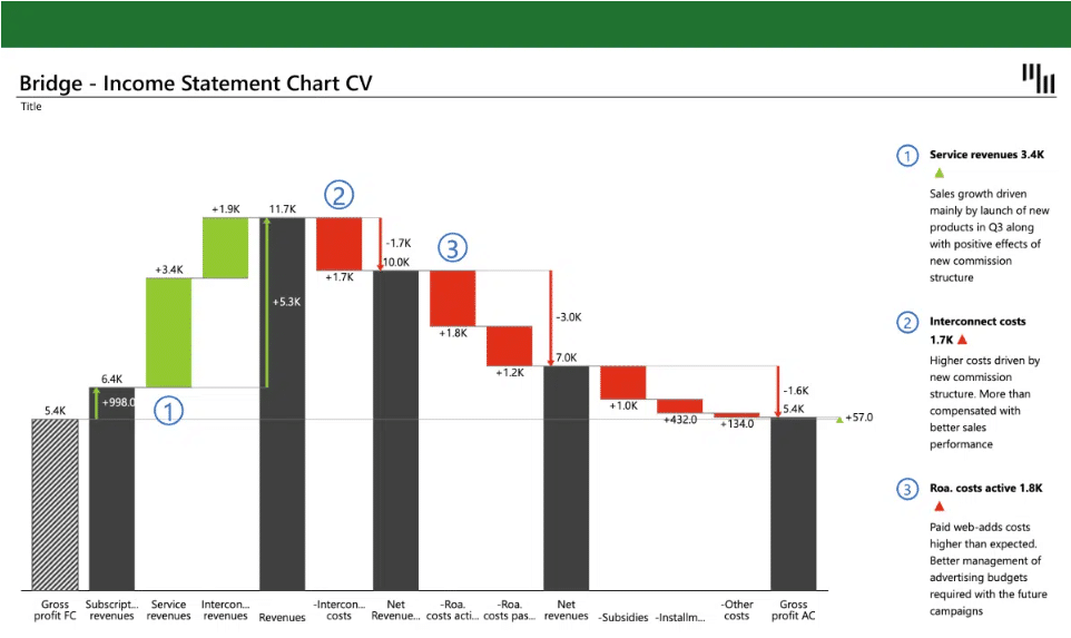
Use Zebra BI visuals for Excel: Get all of the above-mentioned features and more within one visual: automatically calculated variances, customizable formatting, advanced data visualizations (waterfall charts, for example), data labeling, and other elements of visuals aligned with IBCS, dynamic comments, etc. Read our Knowledge Base article with an overview of these Zebra BI for Excel features.

By implementing these best practices, your Excel spreadsheet will be more professional and user-friendly, ensuring clear communication of the results.

How to Use Conditional Formatting to Highlight Negative Results from Cell Subtraction in Excel

Conditional formatting is an invaluable tool for emphasizing negative results from cell subtraction in Excel. Here's how you can use it:

Select the Cells: Begin by highlighting the range of cells that contain the results you want to highlight.
Access Conditional Formatting: Navigate to the "Home" tab and click on the "Conditional Formatting" option in the toolbar.
Choose the Rule: In the dropdown menu, hover over "Highlight Cell Rules." From the expanded options, select "Less Than".
Define the Rule: In the dialog box that appears, input "0" to highlight all negative numbers.
Choose the Formatting Style: Pick the style you prefer from the options. This could be a specific text color (like red), cell fill color, or font style (like bold). After making your selection, click "OK."

As a result, Excel will automatically apply your selected format to all cells in the chosen range containing negative values, immediately making them noticeable.

Automating the Process of Cell Subtraction with Macros in Excel

Consider automating the process with macros if you need to perform identical cell subtraction operations frequently. A macro is a programmed set of instructions that Excel can execute automatically, drastically reducing repetitive manual tasks.

Record a Macro: Record a macro that performs your desired cell subtraction operation. Navigate to the "Developer" tab and select "Record Macro." If you do not see the "Developer" tab, enable it via the Excel Options menu.
Perform the Operation: Carry out the subtraction operation as you normally would. Every action you take will be recorded.
Stop Recording: Once the operation is complete, return to the "Developer" tab and select "Stop Recording." Your macro is now created.
Playback the Macro: You can replay this macro whenever you need to repeat the same subtraction action. Navigate to the "Developer" tab, select "Macros," find your macro in the list, and click "Run."
Modify the Macro: You can modify your macro for more complex operations if necessary. Access it via the "Macros" button, select your macro, and click "Edit." This will open the VBA editor, where you can alter the recorded steps using VBA (Visual Basic for Applications) code.

By creating and utilizing macros, you can significantly streamline your Excel workflows, saving time and minimizing the possibility of human errors.

Troubleshooting Issues with Calculations when Subtracting Multiple Cells in Excel

At times, you may encounter problems when subtracting multiple cells in Excel. These could range from incorrect results to error messages. Here are several steps to help identify and resolve such issues:

Check Formula Syntax: Ensure that your formula is written correctly. Any syntax errors (missing parentheses, incorrect cell references, etc.) could lead to miscalculations or error messages.
Inspect Cell Formatting: The formatting of the subtracted cells could be causing the issue. Check to ensure the cells are formatted as numeric data types. Text or date formatted cells can interfere with calculations.
Detect Circular References: Circular references occur when a formula directly or indirectly refers back to its cell, causing infinite calculations. Excel typically warns you about this with a "Circular Reference" warning. To locate the circular reference, go to the "Formulas" tab, and under "Error Checking," select "Circular References."
Evaluate Order of Operations: If your formula involves multiple mathematical operations, Excel follows the BODMAS/PEMDAS order of operations. Ensure your operations are correctly ordered, and use parentheses where necessary to prioritize calculations.
Consider Formula Precision: Sometimes, Excel may round very large or small numbers in its calculations, leading to minor differences. If extreme precision is required, reconsider the structure of your formula or the accuracy of your input data.

Following these troubleshooting steps methodically will help you identify the problem and apply an appropriate fix, ensuring your cell subtraction operations work correctly.

Using the SUM Function to Add and Subtract Multiple Cells at Once

The SUM function in Excel is a versatile tool for adding multiple cells simultaneously. However, to perform addition and subtraction in the same operation, you would typically create two separate SUM functions, as the Excel SUM function does not directly support subtraction. Here's how you might do it:

Suppose you want to add the values in cells A1 through A5 and subtract the values in cells B1 through B5. The formula you would use is: =SUM(A1:A5)-SUM(B1:B5). This formula first calculates the sum of A1 through A5, then subtracts the sum of B1 through B5 from that total.

The SUM function can also be combined with IF and AND for more complex calculations. For example, you might use a nested IF function within a SUM function to add only values that meet specific criteria.

Remember that Excel performs calculations from inner parentheses outwards so that the nested functions will be calculated first, then the results will be used in the main SUM function.

Comparison of Different Methods to Subtract Multiple Cells in Excel

Excel provides a variety of methods for subtracting multiple cells, and each comes with its unique advantages. The choice of method primarily depends on your project's specific requirements and the complexity of the data you're handling.

Basic Formulas: These are the simplest and most straightforward methods, best suited for basic and small-scale tasks. An example of this method is =A1-B1-B2-B3.
Built-In Functions: SUM and IFERROR are powerful tools that can handle larger datasets and more complex tasks. For example, =SUM(A1:A5)-SUM(B1:B5) or =IFERROR(A1-B1, "Error: Invalid Input").
Absolute and Relative References: These are ideal when dealing with formulas that will be copied across cells or when the cell reference needs to stay constant.
Custom Formulas: These can be created for more complex tasks where built-in functions may not suffice.

While each method should yield the same result, efficiency and accuracy can vary. Some methods might be faster for large datasets, while others provide more error control. Thus, understanding each method's pros and cons becomes crucial in choosing the right one for your task.

Conclusion

This article covers the basics of subtracting multiple cells in Excel and provides tips and tricks for performing this task efficiently and accurately. Whether you are a beginner or an advanced Excel user, the information presented in this article should help you subtract Excel cells confidently.

While many different methods and techniques can be used, choosing the best approach for your needs and preferences is essential.

Turn numbers into insights with 1 click

Create jaw-dropping reports and dashboards with powerful visualization tools to deliver real insights from your data in record time.

Start for FREE