By Sandra Simonovic • Last updated April 15, 2024 •

AVERAGEIF Excel formula

In Excel, the AVERAGEIF formula is a powerful tool that allows you to calculate the average of a range of values based on specific criteria. This function is handy when you have a large dataset and want to find the average of only specific values that meet your specified conditions.

Understanding the AVERAGEIF function in Excel

The AVERAGEIF function in Excel is designed to calculate the average of selected cells that meet a given criterion. It takes two main arguments: the range of cells to evaluate and the criteria to be applied. The syntax for the AVERAGEIF formula is as follows:

AVERAGEIF(range, criteria, [average_range])

The range argument specifies the range of cells that will be evaluated, while the criteria argument defines the condition that must be met for a value to be included in the average calculation. The optional average_range argument can specify a different range of cells to calculate the average.

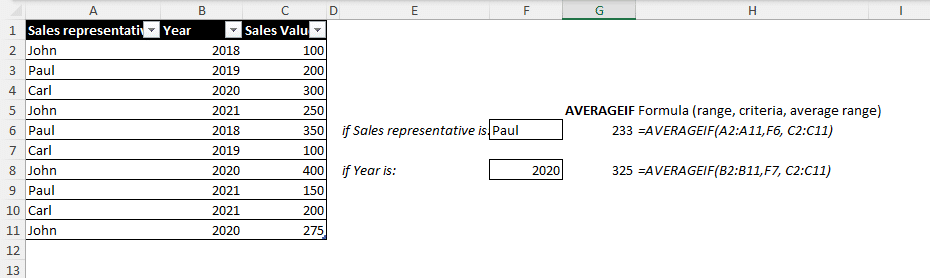
The AVERAGEIF function is a powerful tool in Excel that allows you to perform conditional averaging. It is beneficial when calculating the average of a specific set of values based on a particular condition. For example, you can use the AVERAGEIF function to find the average sales of a specific product in a given region or to calculate the average score of students above a certain threshold.

When using the AVERAGEIF function, it's essential to understand how the criteria are evaluated. The criteria can be a number, a text string, a logical expression, or a cell reference. Excel will compare each value in the range to the criteria and include only those that meet the condition in the average calculation. You can also use operators such as greater than (>), less than (<), equal to (=), and not equal to (<>) to define more complex criteria.

It's worth noting that the AVERAGEIF function only considers numeric values in the range for the average calculation. Any non-numeric values or empty cells will be ignored. If you want to include these values in the average, you can use the AVERAGEIFS function, which allows you to specify multiple criteria.

How to use the AVERAGEIF formula in Excel

To use the AVERAGEIF formula in Excel, you need to follow a few simple steps:

Select the cell where you want the average to appear.
Type the =AVERAGEIF formula, followed by an opening parenthesis (
Specify the range of cells you want to evaluate as the range argument.
Enter the criteria values that must be met to be included in the average calculation.
Add a closing parenthesis and press Enter.

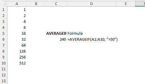
For example, let's say you have a range of values in cells A1 to A10, and you want to calculate the average of only those values greater than 50. The formula would look like this:

=AVERAGEIF(A1:A10, ">50")

This will give you the average of all values in the range A1 to A10 greater than 50.

Using the AVERAGEIF formula in Excel can be a powerful tool for analyzing data. It allows you to calculate the average of a specific range of cells based on a given criteria. This can be particularly useful when you want to find the average of a subset of data that meets certain conditions.

It's important to note that the criteria used in the AVERAGEIF formula can be a number, text, logical expression, or even a cell reference. This gives you flexibility in defining the conditions for the average calculation.

Additionally, the AVERAGEIF formula can be combined with other functions, such as IF or AND, to further refine the criteria for calculating the average. This allows you to perform more complex calculations based on multiple conditions.

By mastering the AVERAGEIF formula, you can unlock the full potential of Excel's data analysis capabilities and gain valuable insights from your data.

Exploring the syntax of the AVERAGEIF formula

The AVERAGEIF formula allows you to use various operators and wildcards in the criteria argument to specify different conditions. Here are some examples:

Using comparison operators: You can use operators such as "<", ">", "<=", ">=", "=", and "<>" to compare values. For instance, =AVERAGEIF(A1:A10, ">=70") will calculate the average of values greater than or equal to 70.
Using wildcards: Wildcards are symbols that can represent any character or group of characters. The asterisk (*) represents any number of characters, while the question mark (?) represents a single character. For instance, =AVERAGEIF(A1:A10, "da*") will calculate the average of values that start with "da".
Using cell references: Instead of manually entering the criteria, you can refer to another cell that contains the criterion. This provides flexibility, as the criterion can be easily changed without modifying the formula. For example, if cell B1 contains the criterion ">=80", you can use =AVERAGEIF(A1:A10, B1) to calculate the average based on the value in B1.

Exploring the syntax of the AVERAGEIF formula

The AVERAGEIF formula allows you to use various operators and wildcards in the criteria argument to specify different conditions. Here are some examples:

Using comparison operators: You can use operators such as "<", ">", "<=", ">=", "=", and "<>" to compare values. For instance, =AVERAGEIF(A1:A10, ">=70") will calculate the average of values greater than or equal to 70.
Using wildcards: Wildcards are symbols that can represent any character or group of characters. The asterisk (*) represents any number of characters, while the question mark (?) represents a single character. For instance, =AVERAGEIF(A1:A10, "da*") will calculate the average of values that start with "da".
Using cell references: Instead of manually entering the criteria, you can refer to another cell that contains the criterion. This provides flexibility, as the criterion can be easily changed without modifying the formula. For example, if cell B1 contains the criterion ">=80", you can use =AVERAGEIF(A1:A10, B1) to calculate the average based on the value in B1.

Using multiple criteria: The AVERAGEIF formula also allows you to use multiple criteria to calculate the average. You can do this by using the AVERAGEIFS formula instead. For example, =AVERAGEIFS(A1:A10, B1:B10, ">=70", C1:C10, "<=90") will calculate the average of values in column A that are greater than or equal to 70 and less than or equal to 90.

Using logical operators: In addition to comparison operators, you can also use logical operators such as "AND" and "OR" to combine multiple criteria. For example, =AVERAGEIF(A1:A10, "AND(>=70, <=90)") will calculate the average of values that are greater than or equal to 70 and less than or equal to 90.