"Oh, how did you do that Power BI DAX trick? How do you do the year-to-date slicer? Can you change the measures dynamically in charts?"
All of these and much more can be solved in Power BI using DAX. Tips and tricks that you'll learn in this tutorial will enhance the usability and the user-friendliness of your dashboards in a really massive way.
Remember the well known open-ended Wh- questions we all learned about in elementary school? The what, the how, the why, the who, the when, and all the rest?
In this tutorial we'll explore the 6 fundamental questions of Business Intelligence:
How much?
What?
When?
Who?
Where?
Why?
Start with an ''Overview''
Note: This Power BI DAX tutorial is based on our 1-hour webinar on the same topic. If you prefer to watch the video, scroll to the bottom of this tutorial, enter your details and we'll send you the webinar recording and all PBIX examples to go along with it.
First, we'll show you Power BI data modeling best practices, which will speed up the development of your dashboard pages and reports, and make them much easier to manage in the future.
Then we'll spend the majority of the tutorial on how to use Power BI DAX in a smart way to supercharge your Power BI dashboards.
Finally, we'll prepare a nice Power BI dashboard that you'll be able to share with end-users and your management.
We'll use a slicer to have a very simple way to switch from monthly to year-to-date results. A single click and you can change the view from monthly values to the accumulated YTD values.
Here we're using just one Power BI custom visual. Everything else is done behind the scenes with Power BI DAX, so you can switch between different views.
We'll use the same technique to switch the shown KPI (from showing revenue to gross profit, for example). You can build multiple pages that take advantage of this technique. It's easy to build different views: monthly views, trends, structured tables, comparisons, etc.
We'll add comparisons to the report, using the three most important business scenarios: actual (AC), previous year (PY), and plan (PL). With them, we can build nice variance analysis reports. The key here is these variance reports are completely dynamic, meaning you can dive into the details with a couple of clicks.
Loading the data
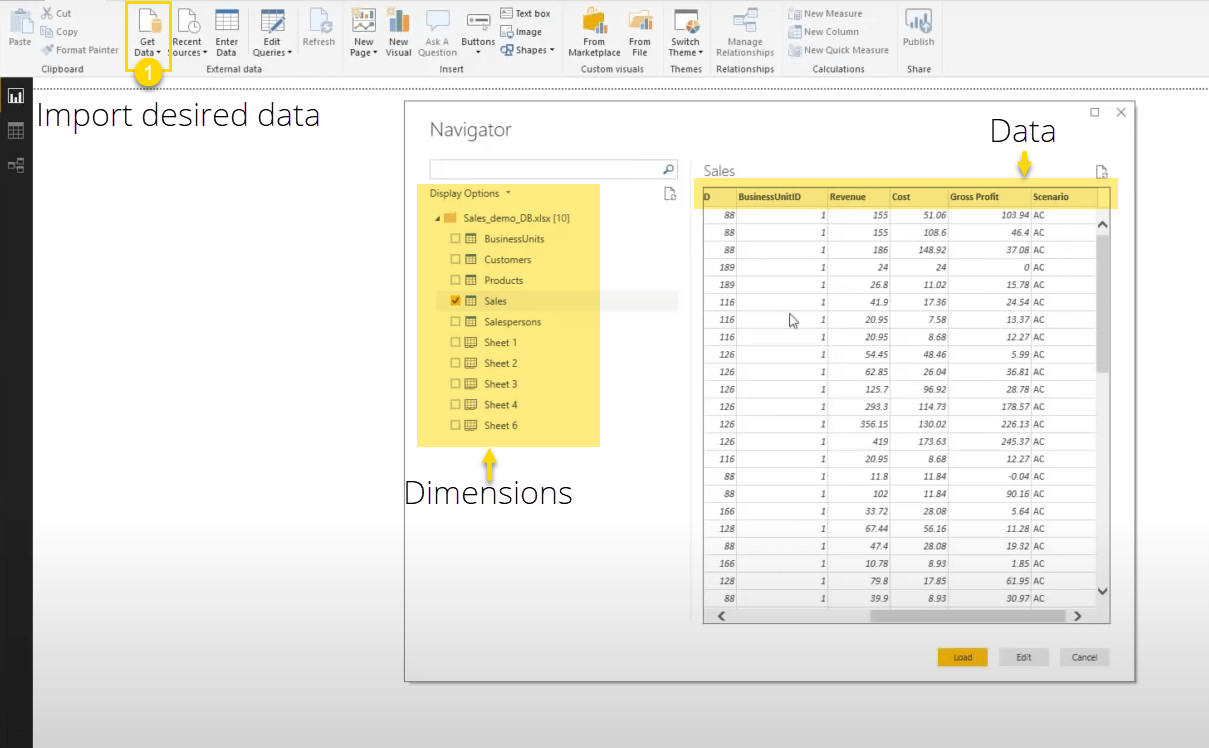
But first, let's start at the beginning. The first step, is to import some data. In our example, we'll import data from an Excel file, specifically a demo sales database.
A key part of this Excel file is a table called Sales. It includes data like date, product ID, customer ID, salesperson ID, business unit ID. It also includes three major KPIs (measures):
revenue,
costs, and
gross profit.
There's also an additional column called Scenario. The Scenario column indicates whether this is actual data or planned data and it's all joined together in the same table. We call this table a fact table.
Also present in this file we also have some typical dimensions tables: business units, customers, products, ...
If all this sounds confusing to you, don't worry. We'll explain everything about fact tables and dimension tables in the next section.
After we load everything into Power BI, we can continue with building a data model. Then we'll dive into DAX and finally, we'll visualize all this data to try and make sense of it.
Data modeling in Power BI
What we're going to build here is the so-called star schema model, the most often used data modeling technique. When you load your data into Power BI, you should always try to organize it in a star schema model.
In a star schema data model, you have one large fact table in the center and all the dimension tables arranged around it and connected to it.
The fact table
The fact table contains all the metrics, measures, and other factual data that are related to a single line item of a transaction, "one row per line in a transaction".
In essence, the fact table contains all of the numerical values. These values can be either
additive (measures that can be added across any dimension),
semi-additive (measures that can be added across some dimensions), or
non-additive (measures that cannot be added across any dimension).
Typical examples of columns in the fact table are:
Revenue
Cost
Quantity
...
A good rule of thumb for fact tables is the following:
A fact table contains data that answers the question How much?.
Additionally, the fact table typically also contains an ID column (like TransactionID) and columns that act as foreign keys for the relationships with the dimension tables:
ProductID
DateID
CustomerID
BusinessUnitID
...
Dimension tables
The dimension tables (or dimensions for short) contain all the descriptive details that explain the data in the fact table.
So, for example, if a row in the fact table contains the quantity and revenue data for a given transaction, a row in the connected dimension table contains the product name for this transaction. A row in another connected dimension table can contain details of the customer: name, address, ... There can be many more dimension tables connected to the fact table.
Here's a simple way to describe the dimension tables:
The dimension tables contain data that answers the questions What?, When?, Who?, and Where?.
Examples of columns in the dimension tables are
Name
Email
Address
Country
Product name
Product description
...
Of course, each dimension table also contains the relevant ID columns (ProductID, CustomerID, ...) needed for relationships with the fact table.
The star schema
Now that we learn what fact table and dimension tables are, let's explore how to put it all together.
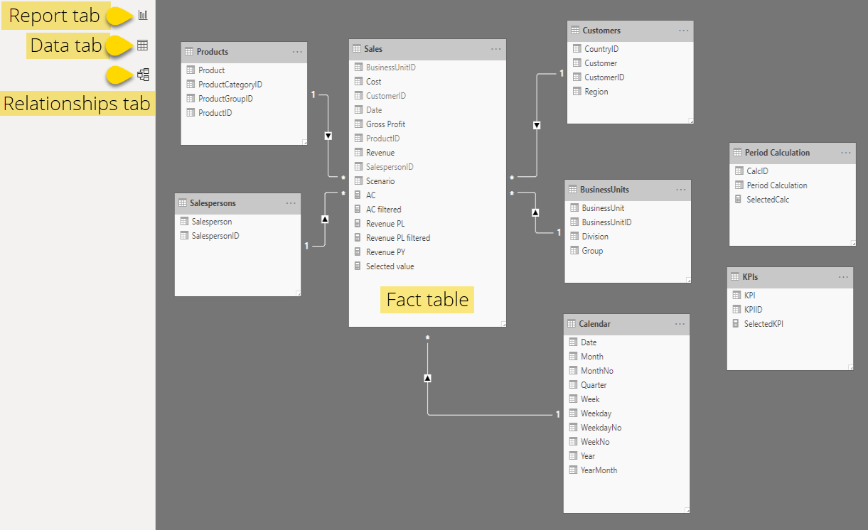
Take a look at this image and you'll quickly notice why its called the star schema:
Note: These relationships were automatically created by Power BI. It has matched them by the column names in the fact table and dimension tables. You can of course create relationships yourself by drag-and-dropping the column names from dimension tables to the relevant columns in the fact table.
In the above example, our fact table in the center is called Sales. As explained in the Loading the data section, it contains Revenue data, Cost and Gross Profit. It also contains the Scenario column and a few ID columns.
Additionally, there are a few calculated measures that we created using Power BI DAX: AC, AC filtered, Revenue PL, Revenue PL filtered, Revenue PY, and Selected value.
We'll explain how these calculated measures are defined a bit later on.
Neatly distributed around the central fact table are 5 dimension tables:
Product,
Customers,
BusinessUnits,
Calendar,
Salespersons.
The connections from the dimension tables to the fact table in the center give the impression of a star, hence the name the star schema.
You'll also notice two other tables on the right: Period Calculation and KPIs. These are the supporting tables and they are not connected to any other table.
The Why
Let's quickly summarize what we've covered thus far.
At the beginning of this tutorial, we set on a journey to answer the 6 fundamental Wh- questions of BI.
We learned that the answer to How much? lies in the fact table and its numerical data. Dimension tables and their descriptive details take care of 4 additional questions: What?, When?, Who?, and Where?.
The only question left to answer is Why?.
The Why of BI. (say that out loud, I dare you 😀)
This is where the fun begins. The Why? is the most important BI question to answer and we'll use two tools that will help us answer it:
Power BI DAX
Data visualization
Power BI DAX will be take up the majority of our focus for the rest of the tutorial. It's in the title, after all. But fear not, we'll cover some interesting data visualization topics along the way as well.
So grab your favorite beverage, buckle up, and enjoy. Let's go!
Power BI DAX trick #1: the calendar
The first thing we need to take care of is the calendar dimension table. This table will contain all of the time series data - the days, weeks, months, quarters, years, days, and also things like weekdays, week number, etc.
A good calendar dimension is the core element of every Power BI data model.
Once your calendar dimension rock-solid, you will have a much easier time creating various comparisons, like actual vs. previous-year (AC vs PY).
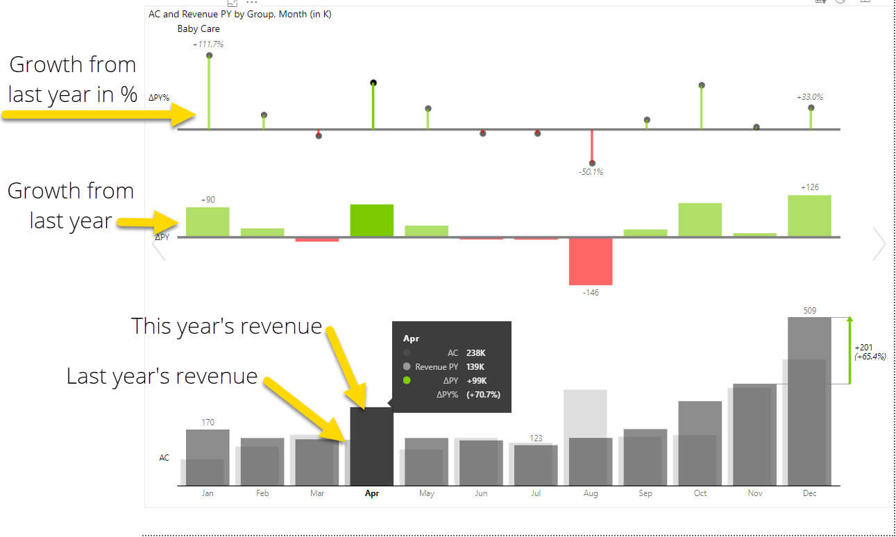
Here is an example of one such AC vs PY report in Power BI. It visualizes this year's revenue compared to previous year's revenue.
This monthly comparison of this year data versus the previous year is a very basic concept in theory, but you need to know your DAX to do this in Power BI.
So let's get to it.
We'll create the calendar dimension from scratch. To add it to the report we'll switch to the data view on the right.Just click New table on the top to create a new table. Name this table Calendar and choose the CALENDAR function, which actually builds a list of dates.
Below is an example of a calendar from the first of January to 2016 to the end of 2018. This will show us a simple column called Date.
Calendar = CALENDAR("2016-01-01", "2018-12-31")
And yes, that's exactly what we already have in our sales table. The difference is that now we have one row per day and we can now add new columns. If you click on the New column button in the top bar, you can add new columns using time functions. The first one we'll do is just called "Year", and we'll just extract the year from the date we already provided. That's really simple to do.
The function YEAR will extract this and simply return the year. The only thing left is to format the year by using the FORMATfunction. To get the year you just type the year and four Y letters. This formula returned the year, like before, but this time it's considered as a text.
"Year", FORMAT([Date], "yyyy"),
Now you can add another column to showcase months. Let's call it "Month", and we'll use the FORMATformula again: Format the date, this time using three M characters.
"Month", FORMAT([Date],"MMM"),
This is how you can build your custom columns which you will use in your reports. You can add the quarter, as well. Use the format date to extract the data and use Q for "quarter". This returns a number between one and four. But, if you want to have values like Q1, Q2, Q3 and Q4, you can do that as well, by adding the letter Q in front of the number and use concatenating.
"Quarter", Q & FORMAT([Date],"Q"),
That's the standard way in Power BI. But there's an even easier way, as shown below. In this case, the backslash displays the letter Q, which is followed by the number of the quarter.
"Quarter", FORMAT([Date],"\QQ"),
There are other functions, like weekday, weeknum for week number, and so on, that you can use to build other columns in your date or Power BI calendar table.
Using CALENDARAUTO
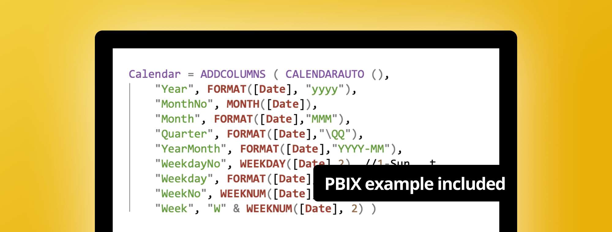
However, there's another way how to do this, and that's with the function called ADDCOLUMNS, which automatically searches for the dates in your database and automatically finds the minimum-maximum date and builds everything automatically. Even better, you can use the ADDCOLUMNSfunction in combination with CALENDARAUTOfunction.
You can simply copy and paste the whole formula from below. This formula has built the whole calendar table with all the columns and you can tweak individual properties, like should the year be shown as a four or two-digit number.
There is also an option to build your calendar dimension in Power Query, which is another part of Power BI.
You can now use the calendar dimension that we just created instead of the date field from your sales table. This allows you to be much more flexible. For example, you can now say: "I want to see my sales by year."
The last thing to do is to link the new dimension to your data, which you can do by going back to the model view. Click on the Date field within the Calendar table and just link it with the Date field in the Sales table, using drag-and-drop. You should now hide the Date field in the Sales table by right-clicking because we will not use it in the report anymore. Instead, we'll just use the date from the calendar table.
If the order of years is showing in the descending order, you can switch to your field that you want to sort by, and select Sort Ascending to sort the years correctly.
In the above animation you'll also see that when you drill down to show revenue by months, the months will be sorted alphabetically instead of chronologically.
You need to tell Power BI how to sort the months. These are things that look completely obvious to every Excel user but these are real, real challenges that people are facing when they start using Power BI.
You can solve this straight from your report view by going to Column tools and select Sort by column button. You will find your MonthNo column from your calendar dimension. Click on that and the months will be sorted correctly.
Power BI DAX trick #2: the PY measure
We are now able to explore, visualize and analyze these relationships by going back to the report view.
On the right side of the report view, under Fields, you can select, for example, the Revenue and the Date fields. Now we are actually starting to do some sort of analysis with native Power BI visuals. Below can see the trends based on the yearly values and you can even drill down into it. You can see that there's sort of a yearly trend and that revenue is growing over time, but it's really hard to see what is going on. The labels are not very intuitive and clear.
But this is really not an analysis. What we need, first of all, is to add a comparison. Once you compare one value with another value you start to understand what is going on: is this better or worse than planned? How much better, how much worse? Is it better than the growth from the previous year?
Once you have a comparison in your model, you can actually start with your most important job: the analysis.
Visualizing data with Zebra BI for Power BI
Remember how we said we'll use two tools to help us find the answer to The Why of BI? Power BI DAX and data visualization.
We already went quite deep into DAX when we built the calendar dimension.
Now it's time to spend some quality time on data visualization.
Why? Because most people would need no more than a couple of seconds to understand the key message of a well-designed Power BI dashboard.
Compare that to a couple of minutes it would take them to discern anything from a messy spreadsheet.
So, data visualization = good. But that's not to say that all data visualization is good data visualization. Not at all.
So stick with Zebra BI and you'll be fine. 😀
Note: You can import the Zebra BI custom visuals for free from the Microsoft AppSource.
We can now we can start analyzing data and start building dashboards.
Let’s analyze the revenue by month, and use the year as a slicer. This allows the end-user to choose the year, which is a basic requirement for many reports. Drag the Year measure onto the canvas and switch to the Slicer visualization and set it as a dropdown.
But this is still not enough, because all we can do now is to change the year and see the monthly development. The only thing that you can really do here is to see if the results are better in the summer or in winter and trends and outliers. What's more important, is to compare our actual revenue with the planned revenue. We can do this because there are actually two types of values in the sales database. There are plan values and actual values.
So, first of all, we need to separate actual results from the plan by creating a new measure.
Let’s create a measure called "Revenue AC filtered" which shows the actual revenues. You can do this by first running a SUM function on all the values of the revenue column. To filter it by actuals you can use the CALCULATE function. The formula will first take the sum of the revenue column and with the added FILTER function, you can actually filter the sales table. Type in Sales and use the Scenario column to filter rows with AC.
Here is the end formula:
Revenue AC filtered = CALCULATE(SUM(Sales[Revenue]), FILTER(Sales, Sales[Scenario]="AC"))
We can now use this measure in the chart. For this example, we are looking at the actual sales in December of 2017. But we can easily do more. We can start by comparing this year to the previous one.
Remember the calendar dimension that we created earlier? You can now actually add another measure to calculate the value for the previous year. Just take the actual revenue and shift the year by one to look at the past year. You can do this by using the CALCULATE formula again:
This takes the actual revenue, which we just calculated before. Now we will use the DATEADDfunction, which is, in a way, most versatile and safest to work with. There are other formulas you can try, like PREVIOUSYEAR, which, while easy to use, has some caveats. You can also use the SAMEPERIODLASTYEAR, the PARALLELPERIOD and a few others.
Now you have the basic model in Power BI to start building your comparisons and you can add this revenue from the previous year into the visual. Now the magic starts to happen. Only now can we actually start building meaningful reports in Power BI.
Variance analysis in Power BI
The visual has changed completely because now our visual understands that you are working with two values. You have actual values and the previous year. Our visual calculates the sum of the previous year on the left side and the actuals on the right. The visual already calculated the growth and now everything else happens automatically. The growth from previous year is expressed in percentages and if you click it, you will have it in absolute values, or you can click again to display both. Now you have year over year values for each variance for each month.
You can just simply switch between different types of charts by clicking on the arrow on the side of the chart and just do a simple line comparison. Or you can use area charts and column charts with different types of layouts. If you have very limited space, you can just use a column chart with the variances.
When you have a very small chart and other things around it, the user can simply open a chart in the Focus mode where everything is big and the relative variances are calculated.
If you're interested in learning more about variance analysis in Power BI, here's a full 1-hour webinar on the topic: Mastering Variance Reports in Power BI.
Combining multiple visuals
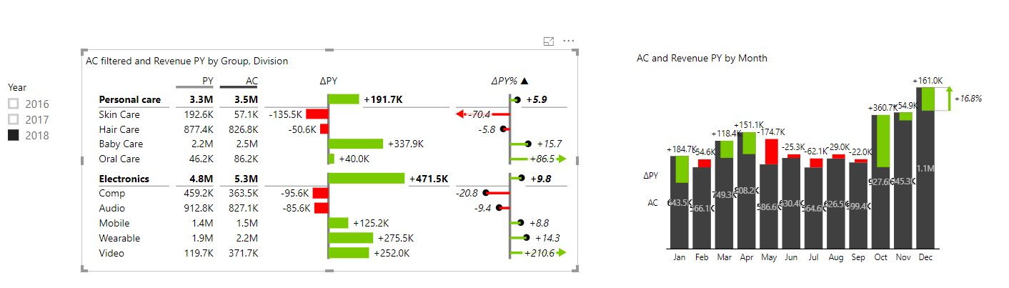
Now we can start building dashboards by combining multiple visuals. We'll use the group of business units and do the comparison of actual versus the previous year. In a single chart, you have the actual, variance to the previous year in absolute numbers and in percent. You can do very interesting analyses already with the two visuals. For example, you can sort and see the worst performing business units and then click on it to see the details per month.
As you may have seen, we have very different business units here: baby care, wearables, audio hardware, etc. Since this is a company that deals with different types of businesses, it would help to add another hierarchy level. Add the Division field into the Category to understand this business better.
And so we have a split electronics and personal care, two completely different businesses. You can now click on an item to see the result for electronics, the wearables and mobile products, etc. An even better decision is to not just have one chart on the right but to present all the business unit groups there. You can do this by adding the business units to the Group field of the chart.
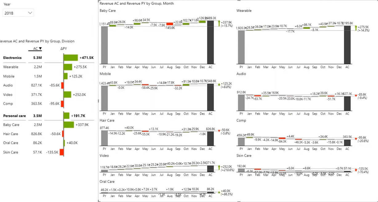
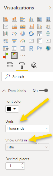
The single chart turned into small multiples and you can see all business units at once. The waterfall chart will look much, much better if you clean it up with proper labels and units. For example, you can show values in thousands. It's much better to just use the K, M, and B suffixes, which the Zebra BI visuals always put in as default. When you change the display units to thousands, you can show the K in the title instead of for each value. Simply pick the option title in the Show units in the field on the right. Now we have revenue and revenue versus previous year comparison shown in K. You can also reduce the number of decimal places or, in some cases, reduce the label density, to make things cleaner.
Some charts also need a little bit more space. You can control this by setting the category width by setting a fixed category width. This allows you to determine the exact width of your columns. Now you can analyze data to just see all the business units or just look closely at what's going on within electronics.
If you have data visualization challenges (like big and small charts side-by-side), you can use the "auto" layout in small multiples. The automatic layout will try to see if there are some large values and will try to arrange other charts around it for a better placement. You can also set the so-called largest-first algorithm, which will take care of really big charts. This usually provides better results if you have large differences between data categories.
Power BI DAX trick #3: the YTD switch
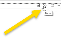
This chart is already starting to make sense but we need even more flexibility. The next thing would be to create the year-to-date switch. But first let’s add a slicer for the month. The user can now select the desired month. Of course, the slicer will filter all visuals on the page, so when you switch to, for example, September, the table part of the dashboard is okay but the trends are broken. To fix this select the slicer, select Format settings in the top bar, and select the Edit Interactions button.
Now turn off the interaction for the visual with the monthly trend. You want this slicer to control everything but the time series, so when a month is selected, it's not affecting the time series. This is the simplest way to control which visuals are affected by a slicer.
Now we need the switch. The switch is used so you can look at data for August or August year-to-date.
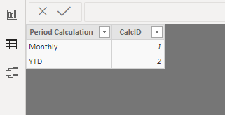
We can do it in the model view, where we'll add another table for the monthly versus year-to-date switch. This is called a disconnected table because it's not having any relationships with other tables. We'll add the table by clicking Enter data at the top bar and we'll just add another table which we can call Period Calculation.
In the first column, we will be inserting the period calculation, and the second one will be a number and we'll just call it CalcID. We'll put monthly in the first column. This is option number one. Option number two is YTD. We created this little table that you can see below and it should be placed somewhere near your calendar.
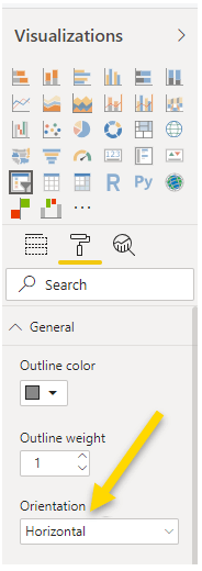
When you go back to your model you have the period calculation column in the Fields. Let’s add the Period Calculation to the dashboard. You now have monthly and year to date options. Change this visual to a slicer and change the orientation to horizontal.
Now we have a button to switch between monthly or year-to-date values. At this point nothing is happening when we click the buttons, because they are not related to other visuals, so you need another Power BI DAX trick.
Create a new measure and call it Selected calculation which will simply return the CalcID of the currently selected button. You can do this by using the MIN DAX function. You can see the full measure code below:
SelectedCalc = MIN('Period Calculation'[CalcID])
Just drop this into your report and display it as a Card visual. When you now use the buttons, the number in the card visual will change. But, how will we link this to the model? First, go back to my Revenue AC measure, which, at the moment simply returns the filtered column from sales. We will rename the measure and call it Revenue AC filtered. Now add a new measure that will take into account the selected calculation and if the value is 2, calculate the year to date value. Check out more about making and using buttonshere.
This will be the true Revenue AC measure. Just add the function name switch within DAX. In the end, it should look like the function below:
Revenue AC = SWITCH ([SelectedCalc],
    1, [Revenue AC filtered],
    2, CALCULATE([Revenue AC filtered], DATESYTD('Calendar'[Date])))
We evaluate the selected button and then go to a new line by pressing SHIFT + ENTER. When the value is one, the formula simply returns my previous measure, which is now called Revenue AC Filtered.
In the second case, when you need the year-to-date value, so you can use CALCULATE to turn Revenue AC Filtered into a YTD value by adding the DATESYTD function. Within the DATESYTD function, you need to add the date column from the calendar table. The Revenue AC measure now evaluates the selected calculation from the switch and calculates year-to-date, if necessary.
Right now the previous year measure still refers to the old measure, so make sure that it will be calculated from the new one and it'll work for both, monthly and for year-to-date. Remove the old measure from the visual and add Revenue AC instead, which takes into account the monthly, the year to date, and will work across the whole dashboard.
All of this is happening in the same visual and everything else is done with switches and drop-down menus.
Power BI DAX trick #4: the AC vs PL
Right now, we show revenue actuals and the previous year. Of course, we can also do this for the plan. First, we will copy what we did for actuals and simply filter by the plan instead. Click New measure and use the below formula.
Now we also need the dynamic measure for the plan, which, we will base on the formula for actuals. Create a new measure and paste in the below formula:
This measure will return the normal plan in the first option and, in the second option, it'll return the year-to-date values of my plan. Now we have the actual, the plan and the year-to-date. However, all of this is just for the revenue. Imagine if you wanted to do this again for the gross profit, one option is to do all of that again for the gross profit, a different KPI.
You could just copy and paste all measures and adjust them to the other KPI, but if you have three, five or ten measures, that quickly stacks up. Moreover, when you want to use those measures in your report, you need to create another visual, so you need one visual for the revenue, the second one for the profit, and so on. But we can do something else. We will use a switch and just reuse the same measure.
Power BI DAX trick #5: the KPI dimension
In trick number five, we'll use the same idea with the switch, but this time we will use it to switch between KPIs. For example, we want to change the charts to show gross profit instead of revenue.
First, we need to add another disconnected table. Go back to the model view and click Enter data and repeat the whole procedure from before. This time, however, we will call this the KPIs table. My first column is the KPI, and the second one will be the numbers (one, two, three) or KPIID. The revenue is KPI number one. Then there's the cost, which is number two, and the third one is the gross profit.
Load this into your model and you get another disconnected table. You can use this KPI now as another switch by changing it to a slicer visual. You can also make it into a dropdown. Then, create a measure that just returns the selection, calling it, for example, SelectedKPI. Again, use the MIN function, which will return the KPI ID.
SelectedKPI = MIN(KPIs[KPIID])
With this selected KPI you can now switch between revenue, gross profit and costs. If you would like to change the order, since everything is sorted alphabetically in Power BI by default, you select the KPI table and set that KPI needs to be sorted by column KPIID.
Finally, you can create another SWITCH measure called Selected value to return the measure that you want.
The below formula will calculate the sum of the revenue as the first option. The second option will return the cost. Number three is the last one and will return a gross profit. This switch simply returns a different column based on the selection in the slicer.
This is now the Selected value measure. Now, we have to now go back to the filtered AC revenue measure and instead of returning the actual for the revenue, we will return the actual for the Selected value, our new measure. Now, this is not revenue anymore but the actual data filtered using the selected column.
AC filtered = CALCULATE([Selected value], FILTER(Sales, Sales[Scenario]="AC"))
This is AC filtered, and now you just go to the revenue AC and rename it into an AC. This is now your generic actual measure that takes into account the year-to-date and the selection of the KPI.
Creating super effective Power BI dashboards in minutes
Having learned how to answer the 6 fundamental Wh- questions of Business Intelligence you can now create Power BI reports and dashboards in minutes.
Now you can put the slicers in whatever order you prefer, like KPI slicer first, then the month, then the year, and then period calculation. You can also turn off the slicer header of the slicers on the right and keep it completely minimal in order to use the space for something more important.
You can also copy the page and use the same thing for different types of measures. For example, you can add the plan, build the tables and compare previous years and actual plans by including variances that you can just reshuffle around. All this on one single page with only one visual.
You can add details like the business units, add more levels, create a multi-level hierarchy, etc. You can even do crazy things like removing the slicer. Because what happens if you remove the slicer? Everything still works. That's the magic of the MIN function, because even if the slicer is not there, the minimum is still evaluated, and it will return option number one.
What you can also do is, remove the business units and use your KPIs under Group. Put KPIs into the Group data field and you'll get small multiples of the measures. Now you have your revenue and gross profit scaled in a small multiple. This helps you understand the relation of gross profit to revenue. You can also go further and create two-dimensional multiples or even multi-dimensional multiples (what a phrase). Just group by another field, which creates the two-dimensional small multiples.
Below you can see that you can also change the order of elements. Besides having the absolute values for previous year, actual and plan, you can also visualize the variance between them. Just drag and drop column headers to reorder the columns. Then use the slicer technique from above for KPI, month, year, monthly/YTD switches, until you've built yourself a nice variance report you're satisfied with.
Watch video recording & Get follow-along PBIX example
If you'd like to try any of these Power BI DAX tricks yourself, enter your data below to get immediate access to the full 1-hour video recording of the webinar and all PBIX examples used in the this tutorial.
Hi Prabhakar, what exactly do you want to know? Otherwise we have all of our newest updates here on our help center. https://zebrabi.com/help-center/ Greetings, Zebra BI Team


please send me latest updates
Hi Prabhakar, what exactly do you want to know? Otherwise we have all of our newest updates here on our help center. https://zebrabi.com/help-center/ Greetings, Zebra BI Team